Elm – fun with L-System (Part 4)

Series:

1. Algae
2. Pythago­ras Tree
3. Can­tor Dust
4. Koch Curve (this)
5. Sier­pin­ski Triangle
6. Dragon Curve
7. Frac­tal Plant

Last time out we imple­mented the Cantor Dust exam­ple from the L-System wikipedia page. Now, let’s con­tinue our jour­ney and see how we can imple­ment the Koch Curve exam­ple in Elm.

 

Example 4 : Koch Curve

Once again, we will start by defining our L-System:

From here, there are a lot of similarities with our implementation for Part 2, so time for a minor refactor!

We’ll add a shared Path module, and move the common abstractions and helper functions there:

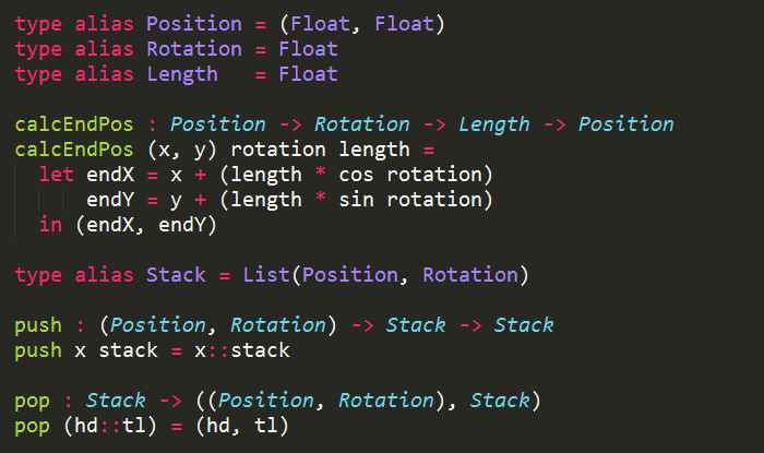
Over the course of the series, we’ll add to this common module to help handle other aspects of drawing our L-Systems.

 

For the Koch Curve, the only thing we really need to implement is the display function to handle ‘F’, ‘–’ and ‘+’:

“Here, F means “draw forward”, + means “turn left 90 degrees”, and – means “turn right 90 degrees”..”

So this was what I ended up with as a 1st pass:

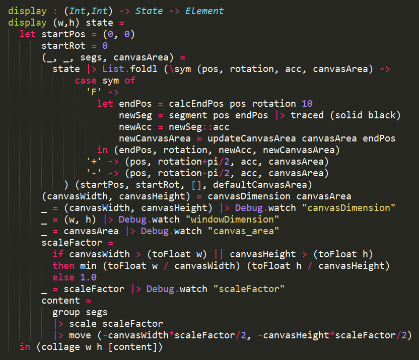
OK, so that was a lot of code to digest, so let’s break it down a bit.

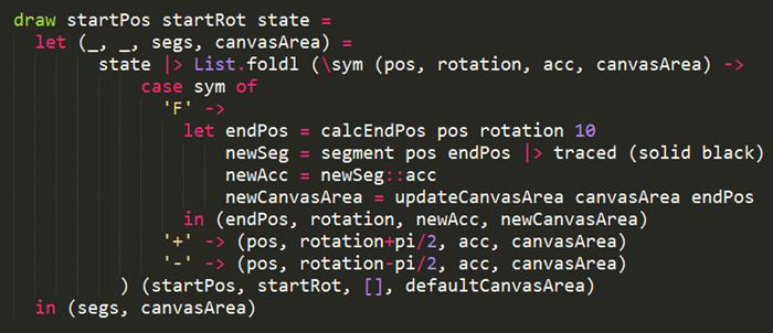
The most important bit of code is here:

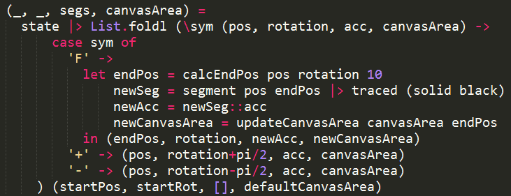
where we implemented the logic for:

• ‘F’ : draw a line segment
• ‘–‘ :  turn left 90 degrees
• ‘+’ : turn right 90 degrees

in a left fold over the current state, using the starting position (0, 0) and rotation angle 0 (radians).

But, what’s this canvasArea that’s passed along?

Aha, good, you caught me! I’ve secretly added a little something to the Path module:

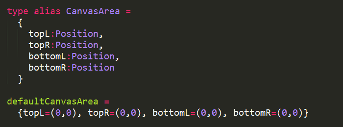
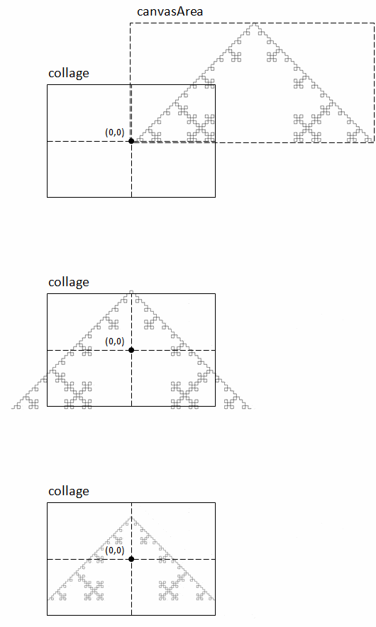
These are to help me track the area that has been drawn on so that I can use this information to scale down and move the completed path later on so that it fits inside the collage and is centred.

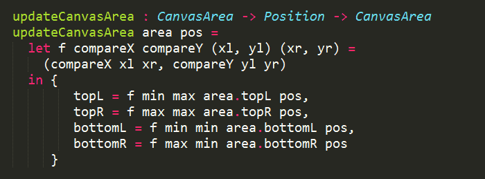
Whenever a new segment has been added the ending position is used to expand the canvas area:

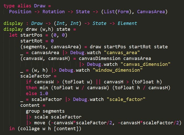
At the end, we work out the scale factor, and move the path to the centre of the collage:

 

As it turns out, much of what’s in the display function is the same across most of the examples, so let’s refactor and move it into the Path module:

and our Koch Curve implementation becomes much simpler:

 

Run­ning this exam­ple in Elm Reac­tor I can get the demo to gen 6, before the rendering time starts to go up noticeably.

 

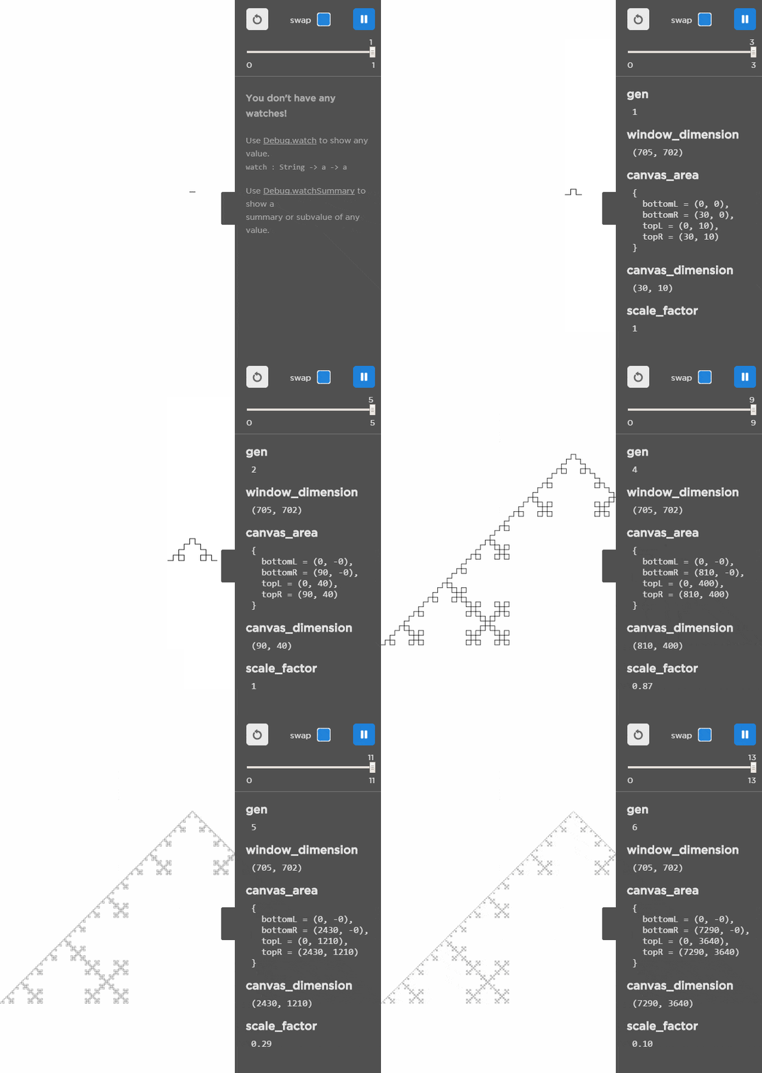
Live Demo (here)

Use LEFT and RIGHT arrow keys to evolve/devolve the L-System.

 

Source Code (here)

 

 

Next : Sierpinski Triangle

 

Links

• Source code for this post
• Live demo